
Join us in building a fintech company that provides fast and easy access to credit for small and medium sized businesses — like a bank, but without the white collars. You’ll work on software wiring million of euros, every day, to our customers.
We’re looking for both junior and experienced software developers.
As data scientists, we design and develop machine learning models, and some of them may appear to be magical. In practice though, when explaining how the internals of these algorithms work to end-users, it turns out they are not that magical at all, but rather quite simple and intuitive. In this post, I’d therefore like to show you that SVMs are not as complicated as they may seem.
As a bonus, all the code to create the datasets and plots from this blog can be found on GitHub and Deepnote.

Being developed in the ’90s, Support Vector Machines are considered to be one of the more traditional machine learning methods. They might not be as ‘new’ as the headline-grabbing algorithms that provide a lot of the AI buzz nowadays, but this does not mean they should be discarded as they are still very popular and performant for several usecases.
My love for SVMs dates back to 2013, some years before Deep Learning suddenly became the next big thing in a time where Tensorflow still had to be released. I used SVMs for my master thesis to perform sentiment analysis on news articles using emotion vectors, and actually achieved a reasonable performance.


What are Support Vector Machines? Essentially, it is an algorithm that tries to find a line that separates two classes of data. Let’s try to explain with an example. Suppose we have a dataset of loan applicants of a Fintech scale-up with two labels: approved and rejected. Each signup has two dimensions - the number of problems & the amount of money on the bank.
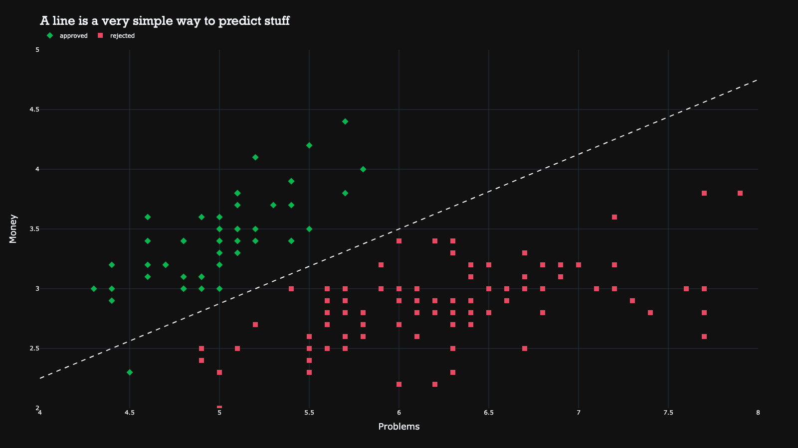
Plotting this data on a graph, with the number of problems on the x-axis and the amount of money on the y-axis, gives the following:

Looking at the plot, it is trivial to see there is a group of customers that is good enough for approval, but there is also a group that is worse enough for rejection. In general, signups with more problems get rejected, unless they have a lot of money on the bank, in which case we may accept them despite the problems.
In essence, what a Support Vector Machine does is to find a line that separates these two classes in the best way possible. Prediction then becomes simple - everything on one side of the line (e.g. above) is approved, and everything on the other side of (e.g. below) the line is rejected. In 2D, the line is a simple straight line, in higher dimensions, such as 3D, it becomes a hyperplane.
As you can see, SVMs are not as complicated as they may seem, they only try to find a simple decision boundary!
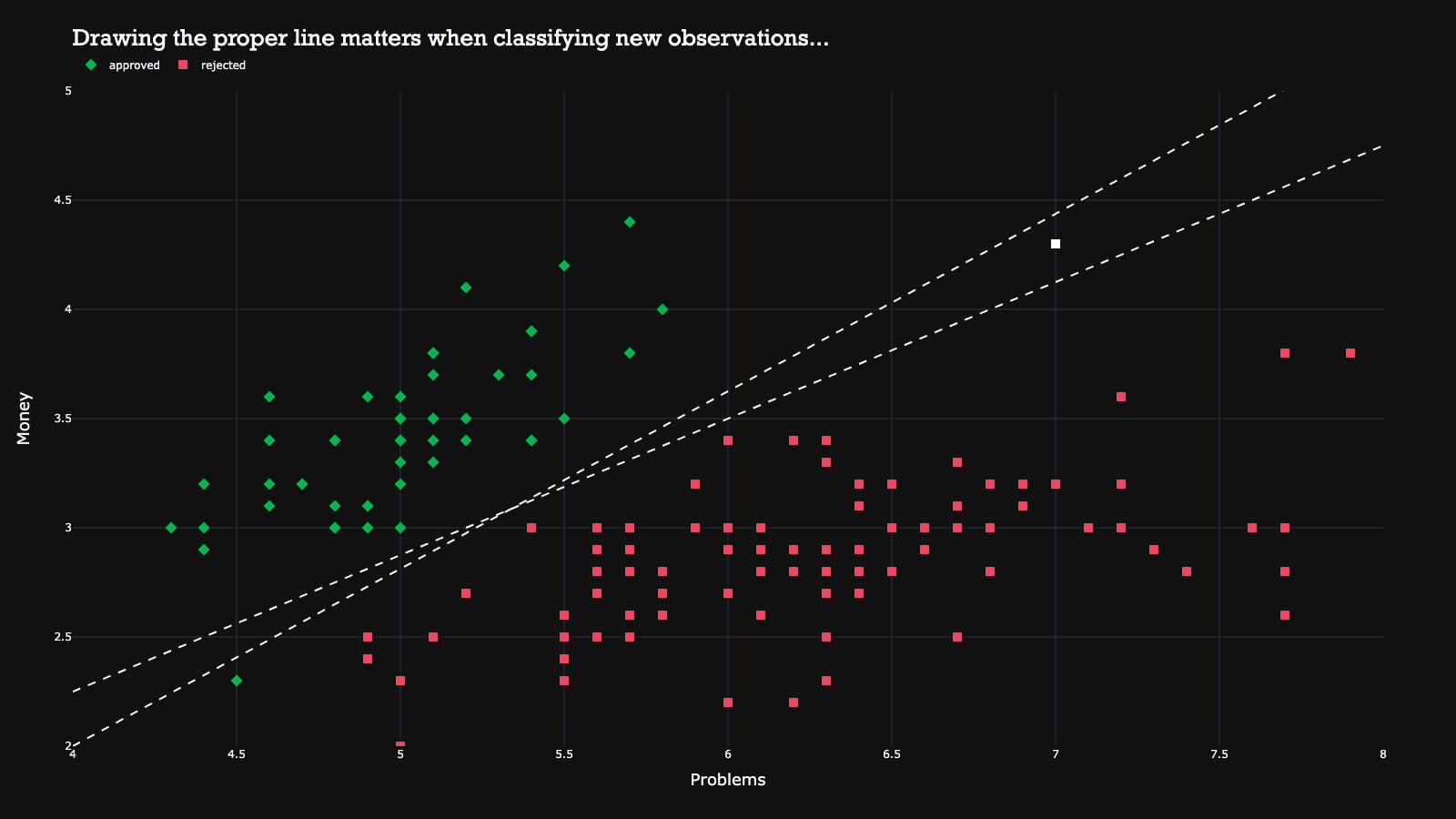
It is crucial to determine the best line that separates the classes, as drawing a random line may not be effective. To demonstrate this, the image below shows an example with one additional signup. Depending on how the line is drawn, the additional signup could either be approved or rejected. Thus, it is important to find the ‘best’ hyperplane that divides the classes. This is exactly what SVMs aim to achieve.
To find the best line, the SVM solves an optimization problem to maximize the boundary or margins around the line. The margin is the maximum space where there are no other observations. By maximizing the margin, the size of the margin denotes how ‘good’ the classes can be separated, which in turn helps to improve classification performance on new observations.
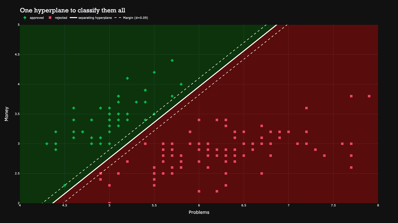
What’s interesting about this machine learning model is that the decision boundary is solely determined by the support vectors. Support vectors are the observations that actually determine how large the margin can be. The other observations are not important because they do not influence the hyperplane directly, for example because they are very far from the line. Hence, the support vectors are the only data points that matter to find the decision boundary, and all others could be removed without the SVM resulting in different predictions.

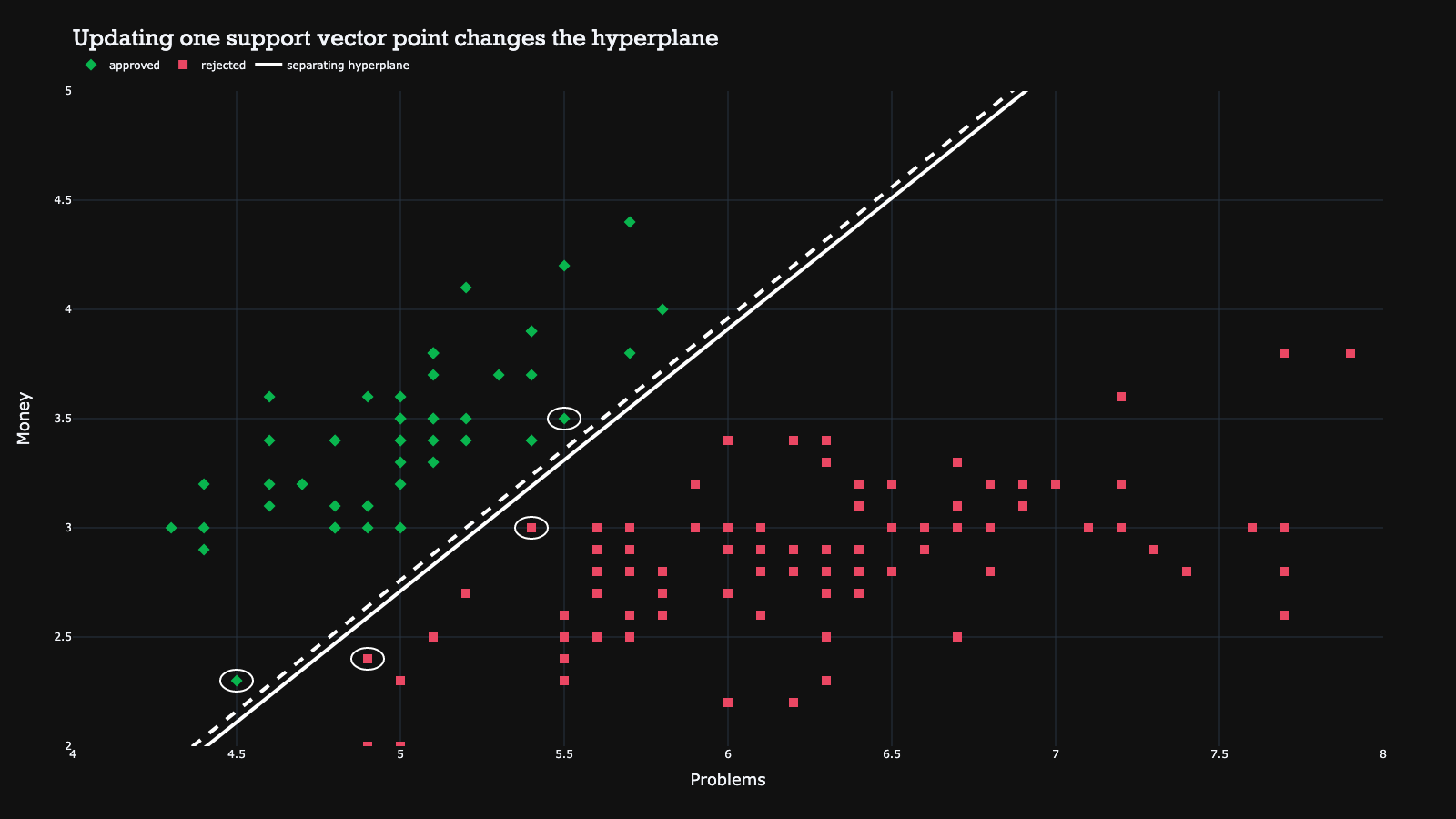
Vice versa, this also implies that updating one support vector changes the entire hyperplane…
In the previous example, a line was drawn to separate applicants, creating a perfect world scenario where no applicant was on the wrong side of the line. In reality, it is challenging to achieve this perfection unless you are using a very simple dataset. In reality, a lot of applicants tend to fall in a grey area, between categories, making it difficult to draw a line that separates all approvals and rejections without any mistakes.

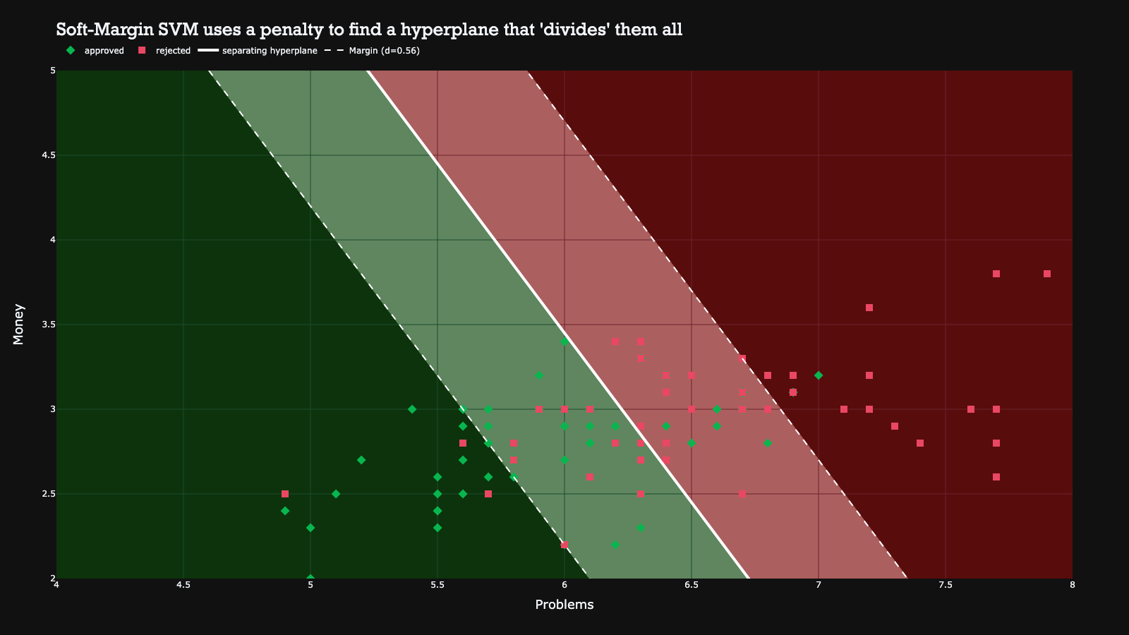
To address this issue, the authors of support vector machines introduced the Soft-Margin SVM (note: the previous implementation was a Hard-Margin SVM). In the soft-margin SVM, observations are allowed to be on the wrong side of the hyperplane, however they will incur a penalty. The SVM then sums all the distances of every point that is on the wrong side of the hyperplane, and considers this a penalty it wants to minimize, while simultaneously maximizing the size of the margin. The result is a hyperplane that balances between finding a good decision boundary while not classifying too many observations incorrectly.
In the example below, the red zone represents all observations that will be classified as a rejection, while the green zone contains all approvals.
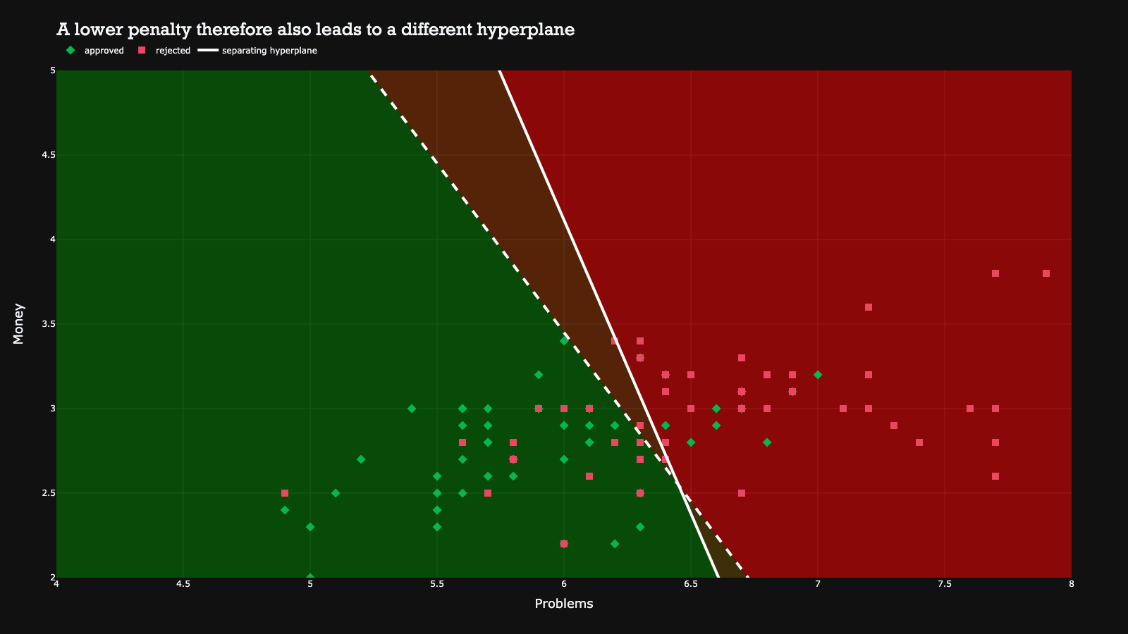
The penalty can be increased or decreased in order to penalize a wrong classification more or less. Depending on the penalty value, the hyperplane can vary. The example below shows how a different penalty value can result in different hyperplanes on the same dataset.
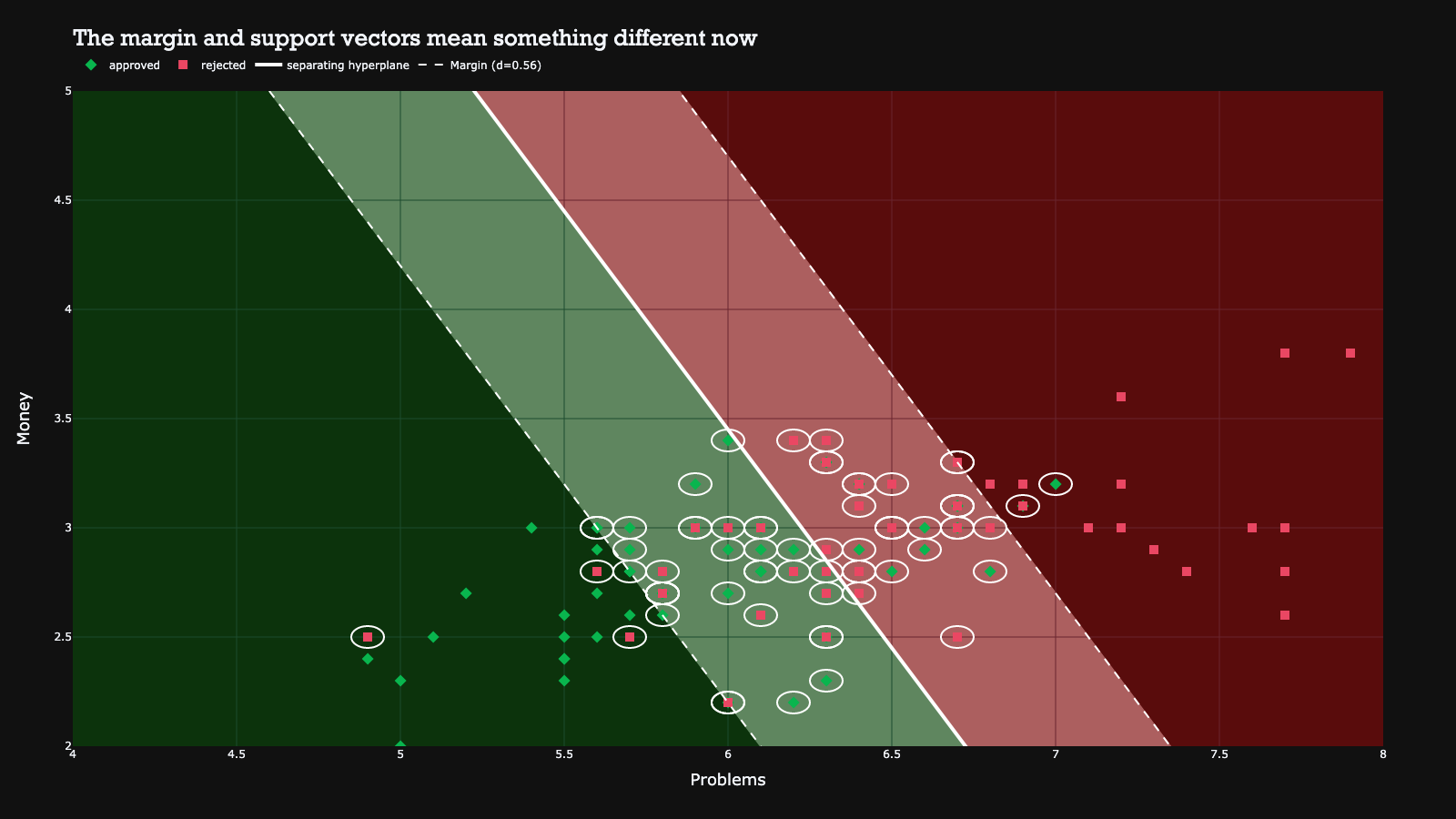
Unlike the perfect separation scenario, we have more support vectors here because each observation that contributes to the penalty becomes a support vector. Removing any support vector would result in a change to the hyperplane. This property is advantageous in practice because our algorithm is not entirely dependent on a few observations.
Unfortunately, there are a lot more complex real-life situations, where it is very difficult to draw a reasonable hyperplane to separate the classes. For example, it’s quite difficult to draw a line that would result in an acceptable separation between the classes in the plot below.
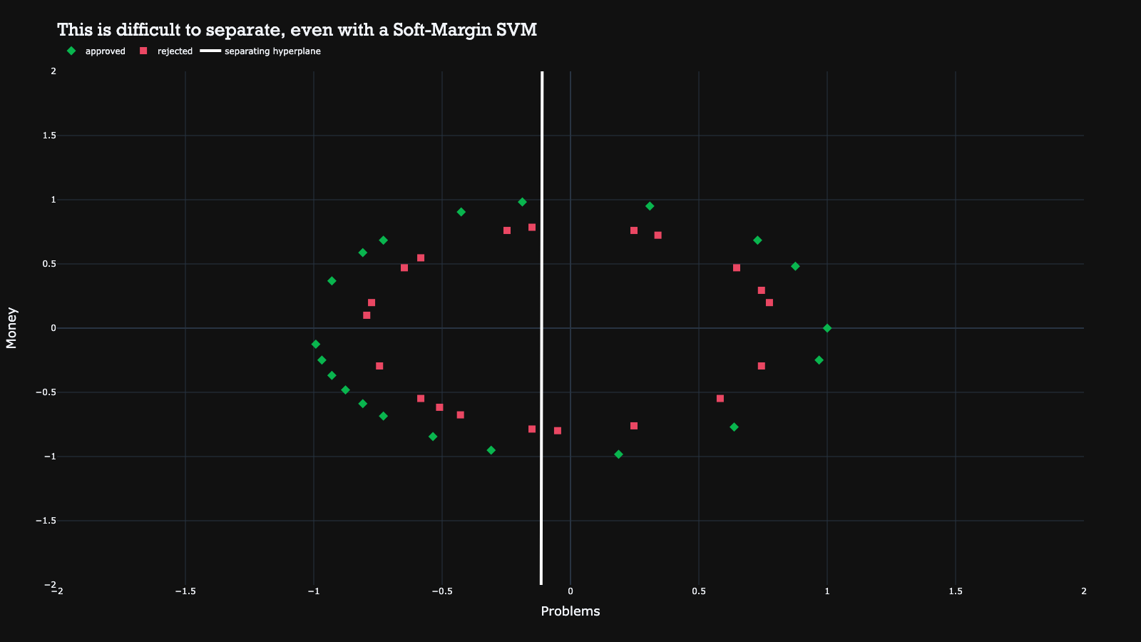
Luckily, there is a still a trick in our toolbox to make them separable by mapping the data to a higher dimension. By doing this in a smart manner, the data becomes separable with a hyperplane in this higher dimension.
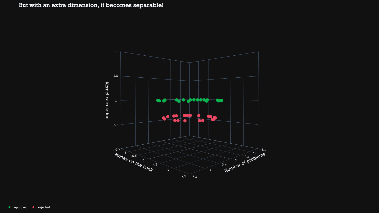
The hyperplane can then be reduced back to the original dimension, resulting in a non-linear decision boundary. This mathematical kernel trick therefore enables us to use non-linear decision boundaries to separate the classes.
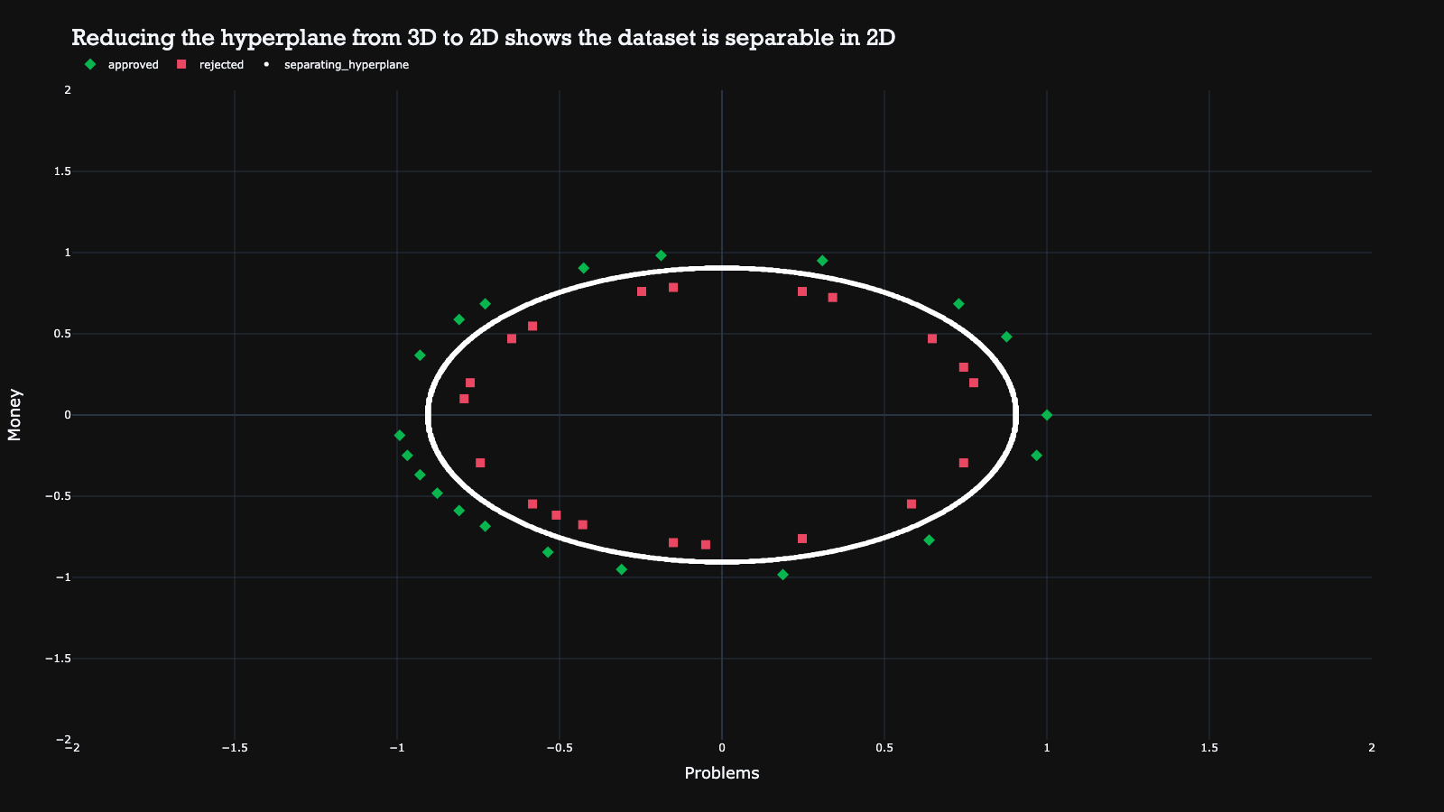
In the example above, a simple transformation from each point (a, b) to (a, b, a^2 + b^2) was used to make the non-linearly separable 2D data suddenly separable in the third dimension. This makes it a very powerful trick for achieving better performance with support vector machines.
In this post I have tried to convey the key principles behind SVMs, and I hope you now think that it’s quite easy and intuitive. Although I only showed you a two-dimensional example in this post, you can use these principles in higher dimensions as well. On a final note, to summarize the pros and cons of SVMs:
While Deep Learning may seem like the way to go in machine learning to achieve good performance, let’s not forget about the tried-and-true methods such as Support Vector Machines. Their principles are still very solid, they are still being used today and can be a powerful tool in your data science toolkit, especially when you want to have more grip on how your model is creating its decisions.
Floryn is a fast growing Dutch fintech, we provide loans to companies with the best customer experience and service, completely online. We use our own bespoke credit models built on banking data, supported by AI & Machine Learning.
